Objectives:
The objectives of this section are:
to introduce you to the various attribute types and the ways they can be split
to present you with an algorithm for creating a decision tree classifier
to determine the best split for a given node
to inform you of the problems that arise with the algorithm and how they are addressed.
Outcomes:
By the time you have completed this section you will be able to:
compare decision trees and decide whether or not they are efficient
explain from a high level Hunts’ algorithms and the difficulties encountered
calculate the impurity of a node by using the measures outlined in this section
compare and contrast the measures of impurity
Efficient Decision Tree Construction
Pacemaker
At this point in time, you should be able to define classification and also be able to identify and define a decision tree. Occam’s razor is another important concept introduced in the previous section that will prove useful in this section, so now would be a good time to brush up on it all if you can’t remember what it is about.
How long do you think it would take you, if you had to use trial and error to find the smallest tree for a dataset that had 240 different attributes? 1 week? 1 month? Or would you just give up and change professions? Fortunately for you (and all of us) there are mathematical measures which determine which attribute should be split to create the most efficient tree. This section is a tad bit more involved and will introduce concepts that are not so introductory, it covers the various attribute types, the ways we can measure and find out the best split and also the different algorithms used to build decision trees. So brace yourself, get a pen and paper because you are about to get your hands dirty.
Attribute Type
Attribute Type: The way we specify a test condition depends on the attribute type, there a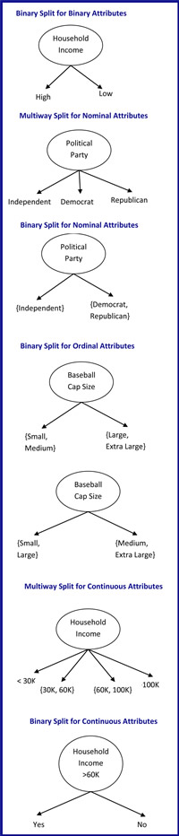 re four attributes types that we can encounter and the way we split them varies for each type.
- Binary: For binary attributes the test condition generates two potential outcomes, so we always use a binary split. Figure 1 is an example of a binary split for a binary attribute.
- Nominal: Nominal attributes are categorical and qualitative and as such they lack most of the properties of numbers. This simply means that you cannot add, subtract or find the mean for a nominal attribute. The values of nominal attributes provide just enough information so that you are able to distinguish one from another. For example, zip codes, gender, eye color are all nominal attributes.
Nominal attributes are expressed in two ways, the first as shown in figure 2 is a multi-way split which uses as many partitions as there are distinct values, and the second is to use a binary split which we obtain by dividing the values into two subsets. The order of the subsets is irrelevant.
- Ordinal: Ordinal attributes are similar to nominal attributes in that they are also categorical and qualitative, the major and crucial difference is that they provide just enough information to order objects. For instance, grades, street numbers, hardness of minerals (good, better, best) are all examples of ordinal attributes.
Ordinal attributes can be expressed as binary or multi-way splits the only difference is that the grouping must not violate the order property of the attribute values. Figure 4 is an example of a correct split for a nominal attribute while Figure 5 is incorrect because the order of the attributes has been tampered with.
- Continuous: continuous attributes are numeric values that have quantitative characteristics. By this we mean that they can perform regular numeric operations on them, like finding the mean, std. deviation, percentages and so on. Like ordinal and nominal attributes, continuous can also be expressed using binary or multi-way splits. For binary, the test condition can be expressed as a comparison test where A<x or A≥x as shown in figure 6. For the multi-way split, the test condition is broken down into ranges as shown in figure 7.

