Objectives
The objectives of this section are:
to introduce alternative methods for generating frequent itemsets.
to compare and contrast the traversal of itemset lattice methods
Outcomes
By the time you have completed this section you will be able to:
explain the general to specific and the specific to general methods for finding frequent itemsets.
compare and contrast the depth and breadth first methods
determine which method is most efficient for a given situation
Introduction
This section highlights the alternative methods that are available for generating frequent itemsets. The Apriori Algorithm that was explained in Section 2 is one of the most widely used algorithms in association mining but it is not without its limitations. When there is a dense data set the Apriori Algorithm performance lessens and another disadvantage is that it has a high overhead.
The way that the transaction data set is represented can also affect the performance of the algorithm. The more popular representation is the vertical data layout which has been shown in previous section examples, an alternative representation is the horizontal data layout. The horizontal data layout can only be used for smaller data sets because the initial layout transaction data set might not be able to fit into main memory. The traversal of the itemset lattice is another crucial area that has improved over the last couple of years. The rest of this section introduces alternative methods for generating frequent itemsets that take the aforementioned limitations into account and try to improve the efficiency of the Apriori algorithm.
Traversal of Itemset Lattice Methods
 General-to-Specific
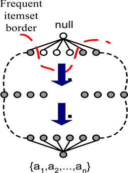
This is the strategy that is employed by the Apriori algorithm. It uses prior frequent itemsets to generate future itemsets; by this we mean that it uses frequent k-1 itemsets to generate candidate k-itemset. This strategy is effective when the maximum length of a frequent itemset is not too long.
Specific-to-General
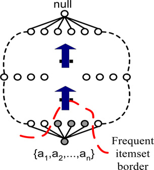 This strategy is the reverse of the general-to-specific and does as the name suggests. It starts with more specific frequent itemsets before finding general frequent itemsets. This strategy helps us discover maximal frequent itemsets in dense transactions where the frequent itemset border is located near the bottom of the lattice.
Bi-directional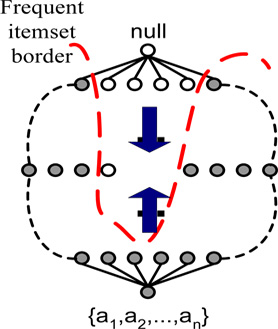
This strategy is a combination of the previous two, and it is useful because it can rapidly identify the frequent itemset border. It is highly efficient when the frequent itemset border isn’t located at either extreme which is conveniently handle by one of the previous strategies. The only limitation is that it requires more space to store the candidate itemsets.
Equivalence Classes
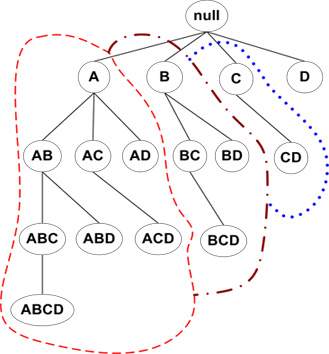 This strategy breaks the lattice equivalence classes as shown in the figure and it then employs a frequent itemset generation algorithm that searches through each class thoroughly before moving to the next class. This is beneficial when a certain itemset is known to be a frequent itemset. For instance, if we knew that the first two items are predominant in most transactions, partitioning the lattice based on the prefix as shown in the diagram might prove advantageous, we can also partition the lattice based on its suffix.
Breadth-First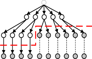
As the name suggests this strategy applies a breadth-first approach to the lattice. This method searches through the 1-itemset row first, discovers all the frequent 1-itemsets before going to the next level to find frequent 2-itemsets.
Depth-First
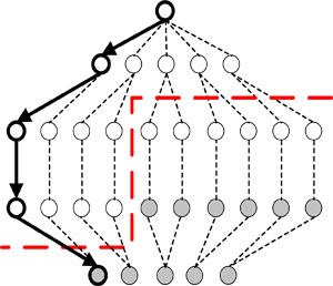 This strategy traverses the lattice in a depth-first manner. The algorithm picks a certain 1-itemset and follows it through all the way down until an infrequent itemset is found with the 1-itemset as its prefix. This method is useful because it helps us determine the border between frequent and infrequent itemsets more quickly than use the breadth-first approach.

